A Real Bar

Here is an examples of a script to make a real bar in a composite disk galaxy with bulge, disk, and halo. There are currently two programs in NEMO that create realistic galaxies: magalie and mkkd95

Initial conditions, integration and visual inspection of the integration as follows:

  magalie disk5 mhalo=0.5
  gyrfalcON disk5 disk5.out tstop=100 step=0.2 kmax=6 give=mxvp > disk5.log
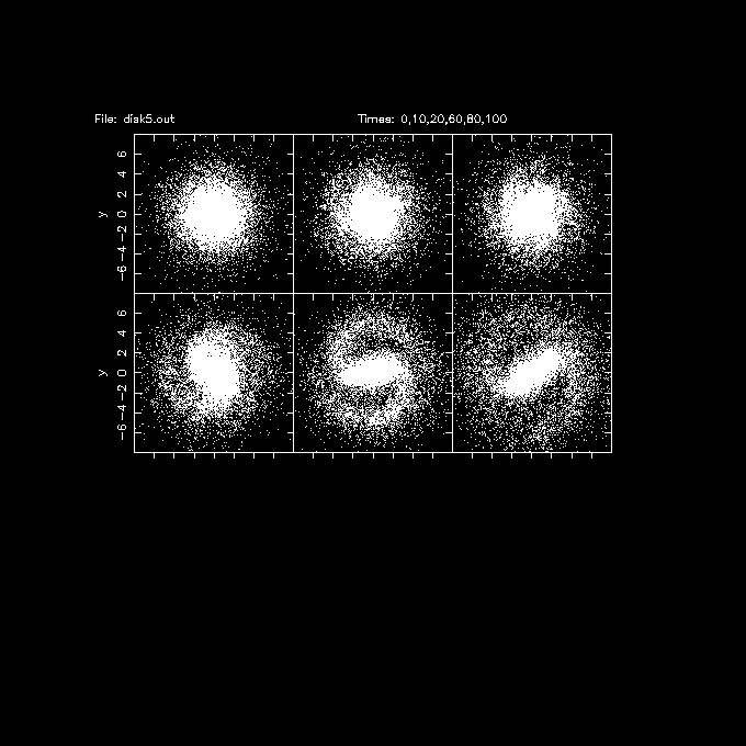
  snapplot disk5.out xrange=-12:12 yrange=-12:12 visib="i<20000" nxy=3,3 times=0,10,20,60,80,100

A few words on the units: V=1 is scaled to the milky way's 220 km/s, R=1 is the (exponential) scale-length of the disk, where the sun is at about R=2.4 (=8 kpc). Hence the unit of time is about 15 Myr (see also units)

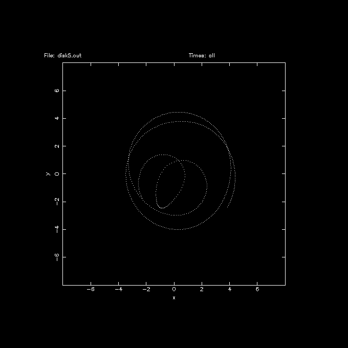
It is instructive to look at an orbit of a star, #8888 in this case. The first 20,000 stars are the disk population.

   snapplot disk5.out xrange=-8:8 yrange=-8:8 visib="i==8888" trak=t

Since the output step was 0.2 units, this corresponds to about 3 MYr in the plot below.

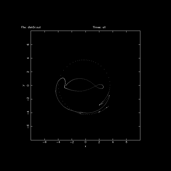
and then aligning the bar E-W in all frames, using snaprect, looking at this orbit in the rotating frame of reference:

   snaprect disk5.out disk5r.out 'i<20000?-phi*phi*phi:0'
   snapplot disk5r.out xrange=-8:8 yrange=-8:8 visib="i==8888" trak=t

Finally, with a bit of hacking from snapinert and table formatting

   snapinert disk5.out disk5.i3tab weight="i<20000?-phi*phi*phi:0" tab=t
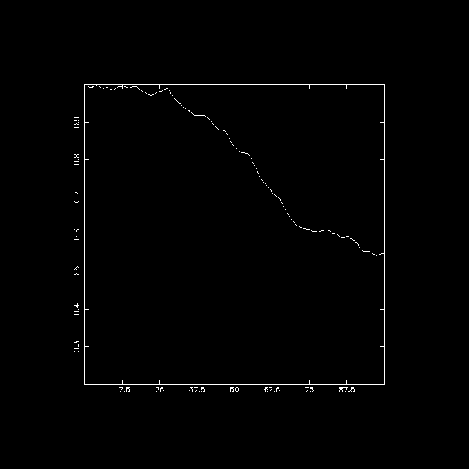
   tabmath disk5.i3tab - "%1,%11,%12,sqrt(%12/%11)" all | tabplot - 1 4 0 100 0.2 1

this plot shows the evolution of the strength of the bar, expressed in something like a density weighted and averaged axis ratio: